

Many individuals discover spreadsheets intimidating. The key to overcoming this? Make it look not like a spreadsheet. Merely hiding the muddle, including interactive menus, and utilizing shapes makes your workbook really feel like a high-end, standalone software that individuals truly need to make use of. Here is every little thing it’s worthwhile to make this occur.
Construct a structured format with high-contrast containers
Use shapes and color-blocking
Fashionable apps use outlined “playing cards” or “widgets” to group associated info and supply visible construction, and you may mimic this professionally in Excel.
Nonetheless, earlier than you begin drawing, choose your entire sheet (Ctrl+A or click on the top-left triangle), right-click a column header, and cut back the Column Width to a small worth (for instance, round 2-3 models). Then, with all of the cells nonetheless chosen, right-click a row header and modify the Row Top to create a dense “graph paper” grid that offers you a lot finer management over the place your shapes and charts sit. To get that premium software program really feel, fill your worksheet cells (or the seen working space) with a darkish grey background.
As an alternative of simply getting into knowledge into uncooked cells, click on Insert > Shapes, choose the Rounded Rectangle, and reformat it with a barely lighter tone that contrasts the background fill. These shapes create a visible nest in your charts and key metrics, giving your “app” the structured depth that individuals count on from devoted software program.
When resizing containers to suit your format, maintain Alt whereas dragging the corners. This snaps the form’s edges to the cell grid, serving to every little thing line up exactly.
For titles, right-click the form and click on Edit Textual content. For dynamic knowledge, insert a Textual content Field over your card, choose the border, and sort = adopted by a cell reference (akin to =Database!$Z$1) within the formulation bar to reflect the worth of that cell.
For consistency, repeat this format on every worksheet.
And determine the lively display screen
A real app would not require customers to hunt by tabs on the backside of the window—it has a persistent navigation rail. You may construct one by putting a tall, slim rectangle on the left facet of your most important sheet.
For performance, place textual content bins or icons inside that sidebar. Proper-click a form, choose Hyperlink (or Hyperlink), and select Place in This Doc to focus on a particular sheet. If you’ve completed creating the menu, duplicate it on all of the sheets, and add a skinny vertical rectangle subsequent to the lively menu merchandise to make it really feel reactive.
By default, Excel turns hyperlinks blue and underlines them, which might conflict along with your design—particularly inside textual content bins and shapes. To stop this from occurring mechanically, go to File > Choices > Proofing > AutoCorrect Choices > AutoFormat As You Kind and uncheck Web and community paths with hyperlinks. This stops Excel from mechanically changing textual content into blue, underlined hyperlinks as you sort, permitting you to use your individual styling with out it being overridden.
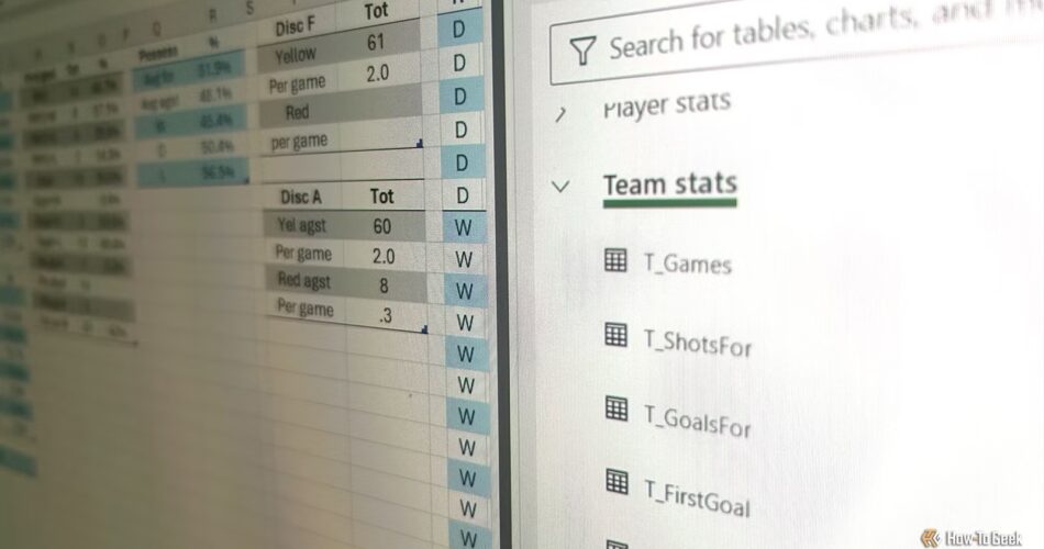
Use Slicers to make knowledge manipulation tactile
In case your “app” requires customers to filter knowledge, do not make them use these small default filter arrows. As an alternative, use Slicers—large, touch-friendly buttons that immediately filter your visuals.
To maintain the “app” look, keep away from connecting a Slicer on to uncooked knowledge. As an alternative, create a PivotTable on a hidden backend worksheet to behave as your engine. Build PivotCharts from that PivotTable, then copy them to your most important interface. If you insert a Slicer for that PivotTable (PivotTable Analyze > Insert Slicer) and replica it to your UI, it acts as a distant management: clicking a button on the Slicer updates the chart, regardless that all knowledge processing occurs safely on a unique sheet.
To make one Slicer management a number of charts directly, right-click the Slicer, choose Report Connections, and verify the bins for each PivotTable driving your dashboard. This creates a unified “command middle” really feel.
As soon as your Slicer is on the interface, it’s worthwhile to eliminate the default styling. Choose the Slicer, head to the Slicer tab, and browse the Slicer Kinds gallery. Decide a darkish fashion that enhances your format, right-click it, and choose Duplicate. Then, right-click the duplicated Slicer and choose Modify to tweak the borders and colours.
Your Excel PivotTable isn’t complete until you add these two pro-level features
Cease treating PivotTables because the end line—add Slicers and Timelines to show your spreadsheet into an interactive dashboard.
Design frameless “floating” charts for a seamless visible circulate
Take away chart borders and axes
Standard Excel charts and PivotCharts have borders and axes, making them seem like stickers slapped onto a web page. To make visualizations really feel extra built-in, you need to strip out the default formatting. Proper-click your chart and choose Format Chart Space. Then, set the Fill to No fill and the Border to No line. In case you’re coping with a PivotChart, click on Conceal All within the Area Buttons menu.
Subsequent, choose one of many chart’s gridlines and press Delete to take away them, and do the identical with the Y-axis labels and legend. Now, click on the Chart Components button (+), verify Information Labels, and select Outdoors Finish.
In brief, the goal is to make the info seem to drift effortlessly inside your structured containers and mix into your software program’s customized UI, and these minor modifications obtain these objectives very quickly.
Proper-click a knowledge bar, choose Format Sequence, and cut back the Hole Width to make the bars wider, thus giving them a extra app-like look.
Conceal the window chrome and ribbon
Pressure a full-screen expertise
Now that your visible interface is constructed, it is time for the magic trick: making the spreadsheet disappear. Up till now, you possible wanted the column and row headings and the formulation bar to ensure every little thing was completely aligned and all formulation had been right, however for the top person, they’re pointless muddle. As quickly as you uncheck Headings and Formulation Bar within the View tab, the “Excel-ness” immediately vanishes, and your customized containers and floating charts take middle stage.
To finish the phantasm, you need to cover the Excel window’s structural parts. Go to File > Choices > Superior, scroll all the way down to Show choices for this workbook, and uncheck Present sheet tabs. This forces customers to make use of the customized navigation menu you constructed earlier.
Lastly, use the Ribbon Show Choices (within the top-right nook) or press Ctrl+Shift+F1 to cover the ribbon for a cleaner, full-screen really feel.
One key to attaining this app-like really feel is making certain the top person cannot see the underlying figures that drive the interface—they solely see what they should see. This mirrors the strategy builders take when designing an app—you by no means see the uncooked code used to make the UI tick. With this in thoughts, when constructing your subsequent mission, organize your workbook into three functional layers: a supply tab for uncooked knowledge, a logic tab for the calculations, and a collection of linked interface tabs that your coworkers can use with out breaking your exhausting work.

- OS
-
Home windows, macOS, iPhone, iPad, Android
- Free trial
-
1 month
Microsoft 365 contains entry to Workplace apps like Phrase, Excel, and PowerPoint on as much as 5 gadgets, 1 TB of OneDrive storage, and extra.
Source link