


For a lot of, the INDEX-XMATCH mixture in Excel is the go-to technique for retrieving a worth from a dataset. Nonetheless, you can even use this dynamic duo to carry out two-way lookups, returning a worth on the intersection of a specified row and column.
This text is aimed toward readers throughout all ranges of Excel experience, rising in complexity because it progresses. When you’re unfamiliar with the INDEX and XMATCH capabilities, proceed studying. Nonetheless, when you already know learn how to use INDEX and XMATCH for one-way lookups, bounce straight to the part headed Utilizing INDEX With XMATCH for Two-Approach Lookups.
How Excel’s INDEX and XMATCH Features Work
Earlier than we take a look at how these two capabilities can be utilized collectively in a single formulation, let’s take a second to discover how they work in isolation.
The INDEX Operate
The INDEX operate returns a worth in a spread in line with the row quantity and column quantity you specify. The syntax is as follows:
=INDEX(a,b,c)
the place
- a is the vary,
- b is the row quantity, and
- c is the column quantity.
For instance, typing:
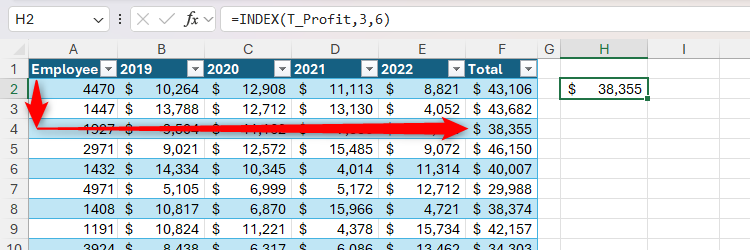
=INDEX(T_Profit,3,6)
into cell H2 returns the worth within the cell that sits on the intersection of the second row and the third column of the T_Profit desk.
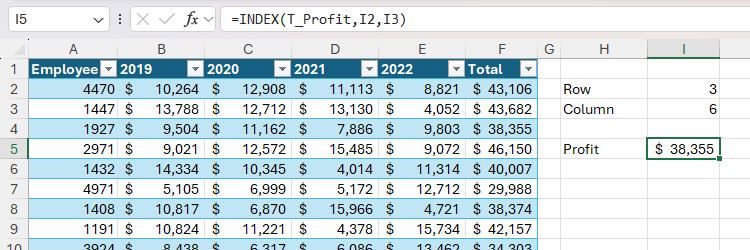
What’s extra, as an alternative of hardcoding the row and column numbers, you may reference cells containing them, making the formulation extra versatile. Right here, typing:
=INDEX(T_Profit,I2,I3)
into cell I5 pulls the row quantity from cell I2 and the column quantity from cell I3.
The XMATCH Operate
The XMATCH operate searches for an merchandise in a spread and returns its place.
When you’re working within the Excel desktop app on a PC or Mac, you might want to be utilizing Excel 2021 or later (together with Excel for Microsoft 365) to make use of the XMATCH operate. It is also available in Excel for the web and on the Excel pill and cellular apps.
This is the syntax:
=XMATCH(a,b,c,d)
the place
- a is the merchandise to search for,
- b is the vary to go looking,
- c is the match sort (0 = precise match (default); -1 = precise match or subsequent smallest merchandise; 1 = precise match or subsequent largest merchandise; 2 = a wildcard match), and
- d is the search mode (1 = first to final (default), -1 = final to first, 2 = binary search the place b is in ascending order, -2 = binary search the place b is in descending order).
It’s possible you’ll be conversant in the MATCH function, which is the predecessor to the extra trendy XMATCH operate. They work in comparable methods, although the default arguments within the XMATCH syntax are extra intuitive than these within the MATCH syntax, favoring a precise match over an approximate one. Additionally, XMATCH allows you to search in both path and use wildcard characters for partial matches—each of which you’ll’t do with MATCH.
On this instance, typing:
=XMATCH(1927,T_Profit[Employee])
into cell H2 returns 3, as a result of the worker ID quantity 1927 is the third worth within the Worker column of the T_Profit desk.
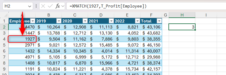
Discover how arguments c and d aren’t required on this state of affairs, as a result of we would like a precise match in a search that runs from the highest of the desk to the underside, and these are the default settings for this operate.
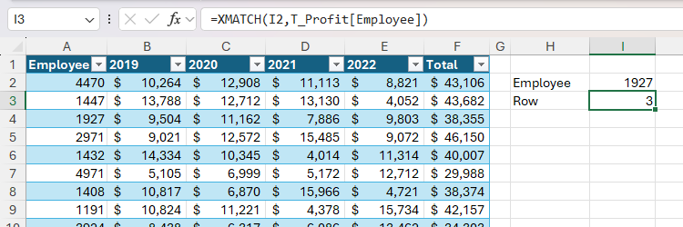
Equally, argument a generally is a reference to a cell containing the lookup worth, that means you may simply change the lookup worth with out modifying the formulation:
=XMATCH(I2,T_Profit[Employee])
the place cell I2 accommodates the worker ID to search for within the Participant column of the T_Scores desk.
Utilizing INDEX With XMATCH for One-Approach Lookups
Whereas the INDEX and XMATCH capabilities might be helpful on their very own, their true potential is realized when used collectively. The important thing to understanding how the INDEX-XMATCH mixture can be utilized to carry out two-way lookups is to first get your head round the way it works in one-dimensional conditions.
As an example you need to view the entire revenue generated by an worker once you sort their ID into cell I2.
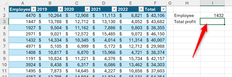
To do that, in cell I2, sort:
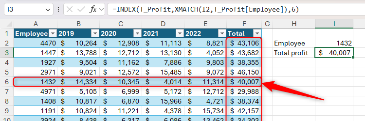
=INDEX(T_Profit,XMATCH(I2,T_Profit[Employee]),6)
the place
- T_Profit is the identify of the desk the place the worth can be discovered,
- XMATCH(I2,T_Profit[Employee]) tells the INDEX operate which row of the Worker column to look in, based mostly on the worth in cell I2, and
- 6 tells the INDEX operate to return the worth within the sixth column of that row.
On this state of affairs, you need not enter the match sort or search mode arguments for the XMATCH a part of the formulation, because the default settings return a precise match and look from high to backside.
However what if you wish to return the worth from one other column, similar to an worker’s revenue in a given yr? That is the place two-way lookups come in useful.
Utilizing INDEX With XMATCH for Two-Approach Lookups
The advantage of utilizing INDEX with XMATCH for two-way lookups is that you could change the parameters in your search with out modifying the formulation. It is because XMATCH identifies each the row quantity and the column quantity, that means you do not have to hardcode them into the formulation.
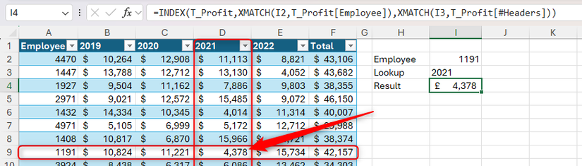
Suppose you need to rapidly learn how a lot revenue worker 1191 made in 2021.
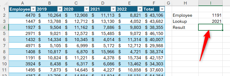
To do that, in cell I4, sort:
=INDEX(T_Profit,XMATCH(I2,T_Profit[Employee]),XMATCH(I3,T_Profit[#Headers]))
the place
- T_Profit is the identify of the desk the place the worth can be discovered,
- XMATCH(I2,T_Profit[Employee]) tells the INDEX operate which row of the Worker column to look in, based mostly on the worth in cell I2, and
- XMATCH(I3,T_Profit[#Headers]) tells the INDEX operate which column of the T_Profit desk to look in, based mostly on the worth in cell I3.
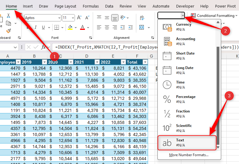
In case your column headers comprise numerical values, like dates, you might even see an #N/A error once you press Enter.
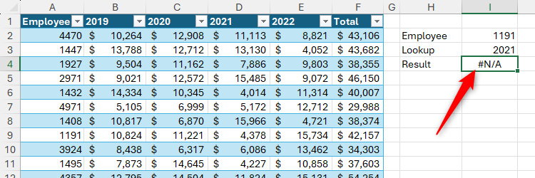
It is because Excel really shops column headers as textual content, even when they seem numeric. So, to make sure you get a like-for-like match between the lookup worth and the lookup array, choose the cell containing the corresponding lookup worth (which, on this instance, is cell I3), and within the Dwelling tab on the ribbon, click on “Textual content” within the quantity format drop-down menu.
Then, choose the cell containing the column lookup worth (I3), press F2 to activate cell edit mode, and press Enter. Now, Excel sees each the lookup worth and the lookup array as having the identical quantity format, so the formulation accurately returns the anticipated worth.
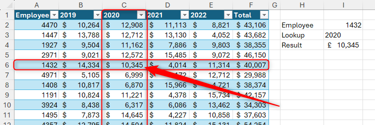
Now, sort totally different lookup parameters into cells I2 and I3, and see the formulation return the corresponding end result.
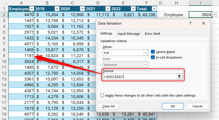
Now that you know the way to make use of INDEX and XMATCH to carry out two-way lookups, you would go one step additional and use data validation to create drop-down menus within the cells containing the lookup values, additional dashing up the lookup course of and making certain you do not by chance enter an invalid worth.
Nonetheless, keep in mind that you simply can’t use column headers as the source of a data validation list. To beat this hurdle, enter direct cell references into the Supply area of the Knowledge Validation dialog field, or name the ranges and reference these as an alternative.
Source link