

One method to give extra which means to your numbers in Excel is to grasp the developments mendacity behind them, and having the ability to take action is essential in in the present day’s ever-changing world. Utilizing Excel’s TREND operate will assist you to determine patterns in earlier and present knowledge, in addition to venture future actions.
What Is TREND Used For?
The TREND operate has three main makes use of in Excel:
- Calculate a linear pattern by a set of current knowledge,
- Predict future figures based mostly on current knowledge, and
- Create a trendline in a chart that helps you forecast future knowledge.
TREND can be utilized to measure efficiency or forecast funds within the office, and you may as well apply it to your private spreadsheets to trace your spending, predict what number of targets your staff will rating, and a number of different makes use of.
How Does TREND Work?
Excel’s TREND operate calculates what can be the road of finest match on a chart utilizing the least-squares methodology.
The road of finest match is calculated utilizing the equation
y = mx + b
the place
- y is the dependent variable,
- m is the gradient (steepness) of the trendline,
- x is the unbiased variable, and
- b is the y-intercept (the place the trendline crosses the y-axis)
Whereas it is not important to know this info, it is helpful for selecting what you need to embody in your TREND system syntax.
What Is the Syntax for TREND?
Now that you just perceive what a trendline is and the way it’s calculated, let’s take a look at the Excel system.
TREND(known_y's,known_x's,new_x's,const)
the place
- known_y’s (required) are the dependent variables you have already got that can assist Excel calculate the pattern. With out these, Excel cannot calculate a pattern, so your enter would lead to an error message. These values would sit on the y-axis on a column chart.
- known_x’s (optionally available) are the unbiased variables that will sit on the x-axis on a column chart, and these have to be the identical size (variety of cells) because the known_y’s reference.
- new_x’s (optionally available) is a number of units of recent unbiased variables on the x-axis for which you need Excel to calculate the pattern. This tells Excel what number of new y-values you need to add to your knowledge.
- const (optionally available) is a logical worth that defines the intercept (worth b in y = mx + b). FALSE forces the trendline to go by 0 on the x-axis, whereas TRUE means the intercept is utilized usually. Omitting this worth is similar as inserting TRUE (regular).
Calculating Your Current Knowledge’s Pattern
It is now time to place this into motion. Within the instance beneath, we’ve got the income for every of the previous few months, and we need to work out the pattern for this knowledge.

To do that, we have to kind the next system into cell C2:
=TREND(B2:B14,A2:A14)
the place B2:B14 are the recognized y-values, and A2:A14 are the recognized x-values. We do not want any new x-values at this level, as we aren’t creating any forecast income knowledge. Additionally, we do not want a const worth, as setting the y-intercept at 0 would yield inaccurate knowledge.
Press Enter after typing your system, and see that the pattern is displayed as an array.

Predicting Future Figures
Now that we’ve got an thought of the pattern of our knowledge, we’re prepared to make use of this info to forecast the next months. In different phrases, we need to full the pattern column in our desk.
So, in cell C15, we are going to kind
=TREND(B2:B14,A2:A14,A15:A18)
the place B2:B14 are the recognized y-values, A2:A14 are the recognized x-values, and A15:A18 are the brand new x-values for the predictive pattern we’re calculating. We have not specified a const worth, as we wish the y-intercept to calculate usually.
Press Enter to see the end result.

Utilizing TREND With Charts
Now that we’ve got all the information as much as the present date, in addition to the predictive trendline for the approaching month, we’re able to see how this seems to be on a chart.
Choose all the information in your desk, together with the headings, and click on “2D Clustered Column Chart” within the Insert tab on the ribbon.

At first, you will notice each the unbiased variable (in our case, income) and the trendline on the x-axis, however we wish the pattern knowledge to indicate as a line.

To amend this, click on anyplace on the chart, and choose “Change Chart Sort” within the Chart Design tab on the ribbon.

Then, choose the “Combo” chart type, and ensure your trendline is ready to “Line.”

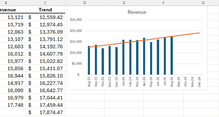
Then, click on “OK” to see your new chart with the trendline displaying as you’ll anticipate, together with as a projection for future months. We have additionally clicked “+” within the nook of our chart to take away the information legend, as it is not obligatory for this chart.
If you happen to aren’t seeking to see future projections in your knowledge, you possibly can add a trendline to your chart with out utilizing the TREND operate. Merely hover your cursor over the chart, click on the “+” within the top-right nook, and examine “Trendline.” One other method to see developments is to use Excel’s Sparklines, which you could find within the Insert tab on the ribbon.
Source link