Nobody told me about these 5 Excel PivotTable tricks—now I use them every day

PivotTables can summarize 1000’s of rows in Excel in seconds, but many individuals nonetheless waste time filtering uncooked knowledge, constructing duplicate reviews, and writing formulation that exist already contained in the device. These 5 missed methods get rid of that additional work and have develop into a part of my on a regular basis workflow.

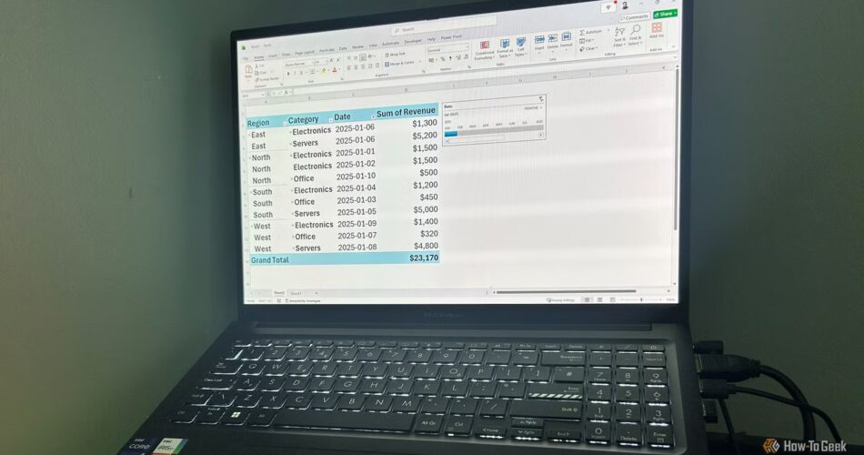
Double-click any worth to see the supply knowledge

Dive deeper into PivotTable data

I found this trick fully accidentally when investigating a sudden spike, and it immediately modified how I troubleshoot and validate numbers.

Suppose you need extra particulars behind one of many values in your PivotTable. Somewhat than flicking between tabs and shedding momentum:

1. Find and double-click the PivotTable worth you need to examine.
2. Overview the newly generated worksheet containing solely the supply rows for that worth.
3. When your evaluation is full, right-click the brand new sheet tab on the backside of your window and click on Delete.

Generate a separate worksheet for each class

Cease copying and pasting separate information

That is the PivotTable function that saved me probably the most time final 12 months.

I used to duplicate PivotTables and waste hours every time totally different folks wanted filtered variations of the identical report. Nevertheless, a devoted PivotTable function handles this complete distribution activity mechanically. For instance, in case your report is filtered by area or supervisor, Excel can immediately generate one worksheet for every class within the filter listing very quickly in any respect.

First, arrange the automation:

1. Drag the specific subject you need to break up into the Filters field of the PivotTable Fields pane.
2. Click on contained in the PivotTable to convey up the contextual ribbon instruments.
3. Open the PivotTable Analyze tab.
4. Click on the small drop-down arrow proper subsequent to the Choices button on the far left.
5. Select Present Report Filter Pages from the contextual drop-down menu.

Then, to generate the sheets:

1. Confirm that the chosen filter subject within the pop-up dialog field matches your goal column.
2. Click on OK to run the sheet technology automation.
3. Click on by means of the newly created worksheet tabs to see the person reviews.
4. To export a selected report, right-click a worksheet tab, then click on Transfer or Copy.

OS

Home windows, macOS, iPhone, iPad, Android

Free trial

1 month

Microsoft 365 consists of entry to Workplace apps like Phrase, Excel, and PowerPoint on as much as 5 gadgets, 1 TB of OneDrive storage, and extra.

Use Distinct Depend to trace distinctive values

Tally gadgets with out duplicates

One of many first main limitations I bumped into with PivotTables was that I could not rely distinctive gadgets as a substitute of simply the overall. Customary PivotTables solely provide a primary rely calculation, that means if a single buyer makes 5 separate purchases, a traditional rely returns 5.

By including the supply knowledge to Excel’s Data Model when first creating the desk, you unlock a hidden distinct rely possibility that ignores duplicate entries utterly.

Begin by initializing Excel’s Information Mannequin workspace:

1. Choose your uncooked supply desk and open the Insert tab.
2. Click on PivotTable to open the usual creation dialog field.
3. Select your vacation spot worksheet location. I have a tendency to put them on new worksheets so the supply knowledge and the PivotTable are cleanly separated.
4. Examine the Add this knowledge to the Information Mannequin field.
5. Click on OK to generate your new PivotTable.

Now, your setup is able to swap your abstract to a definite rely:

1. Drag your figuring out subject into the Values field.
2. Proper-click any quantity inside that newly added column and choose Worth Area Settings.
3. Scroll down the calculation listing and click on Distinct Depend.
4. Click on OK.

The PivotTable instantly updates to indicate a definite rely, that means every buyer is simply counted as soon as per area, no matter what number of purchases they made.

Consolidate messy classes immediately contained in the PivotTable

I typically obtain datasets from different techniques with overly particular classes that must be grouped into broader buckets earlier than they’re helpful for reporting. As an alternative of modifying the grasp database or creating helper columns, I deal with the consolidation immediately throughout the PivotTable itself.

Here is how you can create and clear up customized teams:

1. Maintain Ctrl whereas clicking every particular person textual content label in your rows that belongs in your first customized group.
2. With these gadgets nonetheless chosen, right-click any one in every of them, then choose Group.
3. This motion will initially make the PivotTable look messy, so right-click the leftmost PivotTable column header and choose Develop/Collapse > Collapse Complete Area to tidy issues up.
4. Choose the cell containing the generic group label (reminiscent of Group1), then overwrite the prevailing textual content with a extra comprehensible identify and press Enter.

After repeating the choice, grouping, and renaming steps for the remaining gadgets:

1. Proper-click your newly created mum or dad subject header within the grid.
2. Click on Area Settings.
3. Rename the sphere to mirror the class it represents, then click on OK.

Now all associated gadgets and their related numeric values are grouped collectively, so you’ll be able to rapidly summarize classes, spot higher-level tendencies, and produce cleaner reviews with out manually restructuring your supply knowledge.

Calculate month-over-month development with out writing formulation

Let PivotTables deal with the mathematics

Earlier than I found this calculation function, I repeatedly exported PivotTable knowledge and constructed handbook development formulation that may utterly break every time the information refreshed. The native Show Values As option works completely for month-over-month, quarter-over-quarter, and year-over-year dynamic reporting.

To configure a period-over-period development view:

1. Drag your core efficiency quantity into the Values field a second time so it seems duplicated in your grid.
2. Proper-click any cell inside that newly duplicated values column.
3. Hover over Present Values As, then choose % Distinction From.
4. Set the Base Area drop-down choice to the Month subject created out of your Date grouping.
5. Set the Base Merchandise drop-down choice to (earlier), then click on OK.

Now that the PivotTable efficiently shows month-over-month proportion variations, you’ll be able to click on the header of the duplicated values column and rename it immediately within the PivotTable grid (for instance, Month-over-Month Progress). Since that is solely a show label change, not a change to the underlying calculation, you are positive to rename it right here.

Smarter PivotTables, much less handbook work

I’ve stopped constructing duplicate reviews and writing additional formulation since utilizing these PivotTable methods—they’ve streamlined how I work with massive datasets and made reporting much more environment friendly. Past these 5 workflow upgrades, you’ll be able to take PivotTables additional by adding slicers and timeline filters.